The Emperor Has No Identification
Why asset demand elasticities don’t mean what you think

I wrote recently about a paper that should have embarrassed academic finance more than it did.
The finding was simple and brutal. Two hundred and twelve peer-reviewed stock-return predictors — the output of a five-year review gauntlet at the field’s most prestigious journals — predict returns out of sample no better than a computer mindlessly grinding through 29,000 accounting ratios in search of a t-statistic above two. Decades of theory. Decades of careful storytelling about risk and mispricing. And it bought you nothing a brute-force search wouldn’t have found anyway.
That paper was about prediction. Academic finance, it turned out, fails the prediction test.
I want to tell you now about a paper that does something worse.
It does not go after the predictive wing of the discipline. It goes after the structural wing — the half that doesn’t try to forecast next month’s return but claims, far more ambitiously, to measure the deep parameters of investor behavior. The demand curves. The elasticities. The numbers that tell you how much prices move when a central bank buys bonds or an index fund rebalances.
And it proves — from two assumptions that essentially no one in finance is willing to give up — that those measurements cannot be made model-free from the holdings-and-prices data they are usually advertised as coming from. Not “are hard to make.” Not “have wide error bars.” They are not measurements at all, unless you first smuggle in the very theory they were supposed to test.
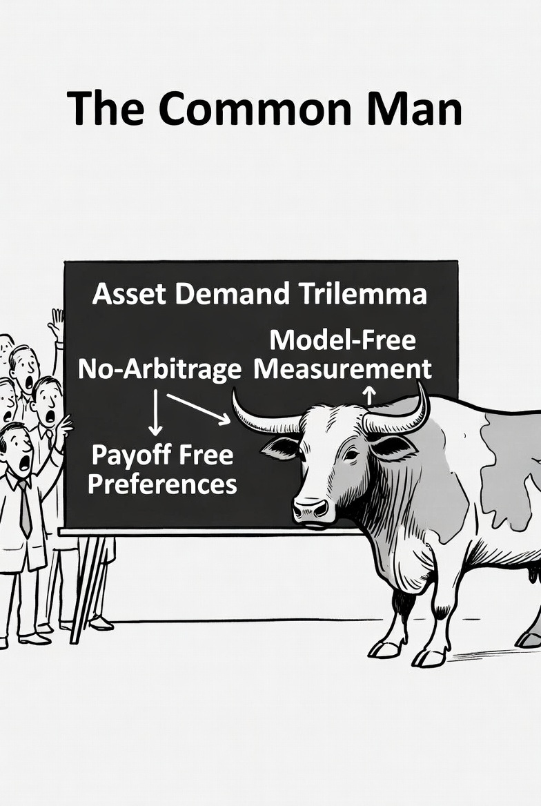
The paper is “A Trilemma for Asset Demand Estimation,” by William Fuchs, Satoshi Fukuda, and Daniel Neuhann. The title gives the structure away. A trilemma is a menu of three items from which you may choose at most two. The three here are: no-arbitrage pricing; the assumption that investors value assets for their payoffs; and the ability to identify structural asset demand from holdings-and-prices data without first committing to a full model. Finance wants all three. It cannot have them. Something has to go — and if no-arbitrage and payoff-based preferences stay, what goes is model-free measurement.
A word on the authors. Two of the three — Fuchs and Neuhann — sit at the McCombs School at the University of Texas at Austin. That happens to be where I earned my PhD, under E.C.G. Sudarshan, with Steven Weinberg on my dissertation committee. The University of Texas mascot is a Longhorn, and its supporters salute it with a hand sign and a cheer: Hook ‘em horns.
What Fuchs, Fukuda, and Neuhann have just done to a research program in their own field is, in precise economic terminology, exactly that.
They put the horns through it.
The thing the paper kills
To see why this matters, you need to know what “asset demand estimation” is, and why a large and serious slice of modern finance has staked its credibility on it.
The idea traces to a 2019 paper by Ralph Koijen and Motohiro Yogo, “A Demand System Approach to Asset Pricing,” published in the Journal of Political Economy. It has been enormously influential. It spawned an entire literature, a small industry of follow-on work, and a vocabulary that has migrated out of the journals and into central banks.
The pitch is appealing. Treat investors the way an industrial-organization economist treats shoppers in a supermarket. Each investor has a “demand curve” for each asset. Estimate those curves from data on who holds what at what price. Out pops a number — the demand elasticity — that tells you how sensitive holdings are to price.
Why would anyone outside a finance department care about an elasticity?
Because the elasticities are load-bearing. They are the inputs to claims you have absolutely heard, whether or not you knew where they came from:
Quantitative easing compressed long-term yields by such-and-such basis points. Adding a stock to the S&P 500 raises its price by some measurable percentage. Markets are “inelastic” — a dollar of net inflow pushes aggregate value up by roughly five dollars — and therefore the rise of passive investing has mechanically inflated stock prices.
Every one of those sentences is an elasticity wearing a coat. Central banks lean on these numbers. The entire active-versus-passive shouting match leans on these numbers. They are not academic trivia. They move policy, and they move capital.
The Fuchs-Fukuda-Neuhann result is that the numbers cannot be identified, model-free, from the data they are supposedly estimated from. Whatever makes the number a measurement of structure, you carried in.
Let me show you why. It is not complicated — and, pleasingly, the argument is essentially a piece of physics.
The dictionary in the middle
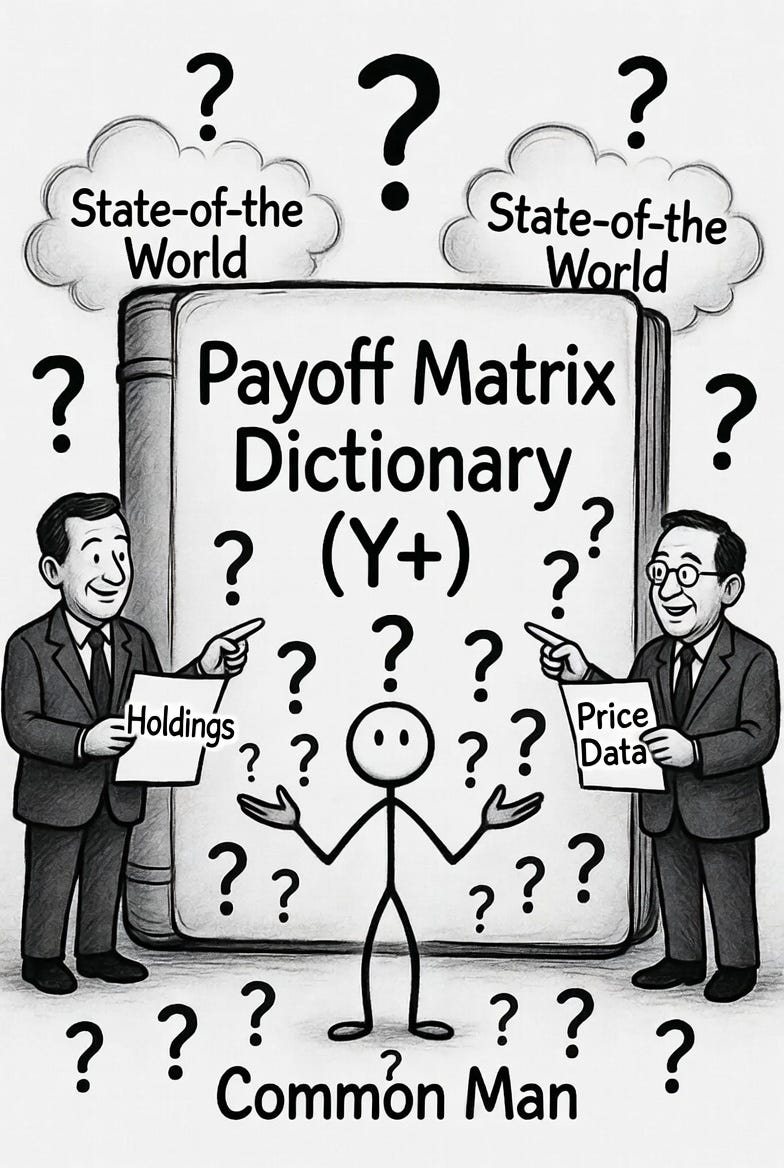
Here is the entire engine of the paper, compressed into a single line. The matrix of asset demand slopes — call it A, the object the econometrician wants — can be written as:
A = (Y⁺)ᵀ D Y⁺
Three pieces. Take them one at a time.
D is fundamental demand. It is what the investor actually cares about. And what an investor cares about, in the standard asset-pricing setup, is not “shares of Apple” — nobody wants Apple stock for its own sake. What they want is consumption: money in good states of the world and, especially, money in bad ones. D describes an investor’s appetite for state-by-state consumption. It is the genuine object of preference.
Y is the payoff matrix. It records what each asset delivers in each possible future state of the world.
Y⁺ is the part that does the damage. It is the Moore-Penrose pseudo-inverse of the payoff matrix — and for our purposes you can think of it as a dictionary. When a matrix is square and well-behaved it has a true inverse, a clean way to run it backwards. Most payoff matrices are neither. The pseudo-inverse is the mathematician’s best available substitute: the closest thing to a reverse gear when no exact one exists. Here, that reverse gear translates the language investors think in — “I want this pattern of consumption across future states” — into the language markets transact in: “therefore hold this particular portfolio.”
Now look at the structure of the problem. Investors have preferences over consumption — that is D. The econometrician observes holdings and prices, and wants to infer A, the slope of asset demand. Sitting between the object investors care about and the object the econometrician wants is the dictionary, Y⁺.
To recover preferences from observed holdings — which is the entire point of the exercise — you need the dictionary.
And here is the paper’s first blow: you cannot have it. Not from the data alone.
Why the dictionary cannot be observed
The payoff matrix Y is not a record of what assets did pay. It is a description of what investors believe assets will pay, across every state of the world — including states that have not happened, and including the future resale prices of the assets themselves.
That distinction is the whole game.
Suppose you have decades of data. Every realized return, every holding, every price. Now I, sitting beside you, change the assumed payoff of some asset in a state of the world that has not yet occurred in your sample. Perhaps it never occurred at all — a market regime that simply didn’t show up.
What have I changed? I have changed Y. Therefore I have changed Y⁺, the dictionary. Therefore I have changed A — every estimated demand elasticity in your model.
What have I left untouched? Every single realized return in your dataset. Every holding. Every price. The data is identical.
Two economies, then, with genuinely different demand elasticities — different answers to “how much do prices move when a central bank buys” — and not one observation that could ever tell them apart. The historical record is mute on the question, because the historical record is a handful of states that happened, and the dictionary depends on all the states, including the ones that didn’t.
This is what an economist means by a non-identification result, and it is fatal to the model-free ambition. Any observed pattern of holdings is consistent with infinitely many combinations of preferences and dictionary. The data, by itself, cannot pick one. It cannot even narrow the field.
You can still write down a model and estimate numbers — people do, every day — but the model is doing the identifying, not the data. The number reflects the theory you chose, not the theory you tested.
The authors put it with admirable bluntness. Estimated demand elasticities, they write, are contingent, model-specific constructs which reflect — rather than validate — a priori assumptions on investor behavior.
Read that twice. The elasticity does not come out of the data. It comes out of the assumptions you carried in. The data’s only role is to sit there, politely, while you confirm what you had already decided.
“But surely a clever instrument...”
At this point every empirically-trained economist reading this has the same reflex, and it is a good reflex. It is the reflex that has rescued a thousand identification problems.
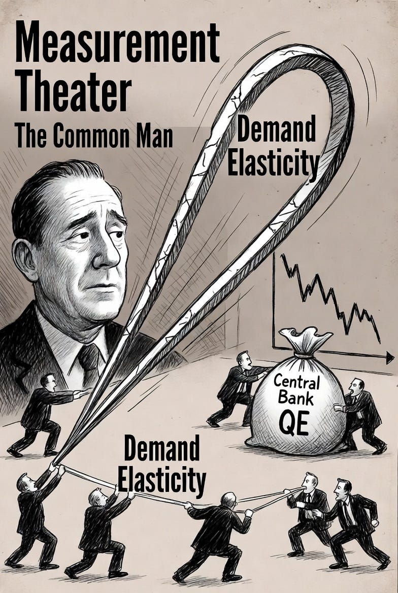
Find an instrument. Find some exogenous shock to the supply of an asset — a Treasury auction surprise, a mechanical index reweighting, a forced sale by a constrained institution — and use it to trace out the demand curve. Supply moves for reasons unrelated to demand; price responds; you read the elasticity off the response. This is the canonical move, and in ordinary markets it works.
In asset markets, the paper shows, it does not. And the reason it does not is no-arbitrage — the single most load-bearing assumption in all of finance.
No-arbitrage says, roughly, that you cannot get something for nothing; that two portfolios delivering the same payoffs must cost the same. It is the assumption underneath every pricing model anyone has ever taken seriously. Nobody is giving it up.
But no-arbitrage has a consequence. If you shock the supply of one asset, its price moves — and no-arbitrage forces the prices of every other asset with overlapping payoffs to move along with it. Overlapping payoffs are not the exception. They are essentially universal: almost every asset pays off in good times, almost every asset pays off alongside almost every other asset in some state. Clean, isolated, one-asset-at-a-time price variation is not something the no-arbitrage world permits.
So your beautiful exogenous supply shock does not nudge one price while the others sit still. It moves the entire interlinked system. The variation you needed — this price changes, all else equal — is precisely the variation no-arbitrage forbids.
And it gets worse, in a way I find genuinely elegant. The paper shows that the price changes a supply shock induces are not merely contaminated. Generically, they point in the wrong direction. The state-contingent prices that should rise, fall. Asking what would happen if only one asset’s price moved is, in an asset market, asking what would happen if no-arbitrage didn’t hold. It is not a hard experiment. It is an incoherent one.
“But surely with enough structure...”
One move remains, and it is the sophisticated one. If you cannot observe Y, impose structure on it. Assume returns follow a factor model — a few common factors plus idiosyncratic noise, the workhorse of modern asset pricing. Surely that pins the dictionary down well enough to make progress.
It does not. And the proof of why it does not is the most physics-flavored thing in the paper.
The authors reach for random matrix theory — the mathematics Eugene Wigner developed in the 1950s because the energy levels of heavy atomic nuclei were too complex to compute, and he realized you could ask what a typical such system looked like instead. Random matrix theory is what you use when the specific details are hopeless but the statistical geometry is tractable.
Applied here, it delivers a result I would call funny if it were not so damaging.
In a large market, the sign of any given entry of the dictionary Y⁺ — not its precise value, just whether it is positive or negative — is asymptotically a coin flip.
A fair coin. You impose your tasteful factor structure, you turn the crank, and whether the dictionary tells you to buy or to sell is, entry by entry, fifty-fifty.
Then comes the kill shot. Take two economies with the identicalfactor structure — same factors, same loadings, differing only in idiosyncratic noise — and their dictionaries agree on sign about half the time. Knowing the factor structure buys you nothing. It cannot, because the instability lives in the geometry of the payoff matrix, not in the part the factor model describes.
The authors then run the experiment. They take real S&P 500 stocks, build payoff matrices from realized quarterly stock payoffs — end-of-quarter prices plus dividends — invert them, and count. Theory predicts the entries of Y⁺ should be positive about half the time. The data says: 50.58 percent.
The coin is fair. The dictionary is noise. There is no factor model clever enough to fix it.
Two halves of the same disease
Step back and look at the two papers together — the first essay and this one.
The first essay went after the predictive wing of academic finance and found that its peer-reviewed forecasts forecast no better than mechanical mining. Theory added no predictive value.
This paper goes after the structural wing — the wing that always considered itself the more rigorous one, the more serious one, less vulnerable to the data-mining critique precisely because it wasn’t fishing for predictors, it was estimating deep parameters. And it finds that the deep parameters were never identified from the data in the first place. The central numbers are model outputs in measurement’s clothing.
Prediction fails. Measurement fails. Same disease, two organs.
And the disease has a name. Academic finance has spent decades borrowing the vocabulary of physics — “structural parameters,” “identification,” “equilibrium,” “elasticity” — without borrowing the part that makes physics work. In physics, the Standard Model committed in advance to a scalar particle with definite quantum numbers and couplings; once its mass was measured, every other property was fixed and falsifiable. General relativity predicted gravitational waves a century before LIGO heard one. The point is not that physics knows everything in advance. It is that real theory sticks its neck out: the data has a vote on whether the theory survives.
Academic asset pricing produces a number — “the demand elasticity is 0.4” — and when you ask what would have to be true in the world for that number to be wrong, the answer is: nothing the data shows. A different modeler, with a different assumed payoff matrix, gets a different number from the same data, and the data has no vote.
That is not a theory in the sense a physicist means the word. It is a very elaborate way of writing down your priors.
A physicist on the receiving end
I want to be personal for a moment, because this paper has changed something for me — and not in the direction you might assume.
For years, people have quoted these elasticity numbers at me.
It happens at dinners. It happens on panels. It happens in my comment section and in my inbox. I will make an argument — that the rise of passive investing is not the mechanical, price-inflating monster it is often made out to be, say — and someone will produce a demand elasticity from the Koijen-Yogo literature the way a lawyer produces an exhibit. The estimates show markets are inelastic. The number says you’re wrong. This is settled.
Until now, my pushback had to come from intuition. From three decades of watching markets do things no demand system anticipated. From a physicist’s itch that a quantity with a published standard error was being treated as a fact about the world when it smelled like a fact about a modeling choice. I believed the numbers could not bear the weight being placed on them. I could not prove it.
Now I can. The proof is this paper, together with a companion: “Demand-System Asset Pricing: Theoretical Foundations,” by the same three authors. In the companion, they take the workhorse logit demand system — the one Koijen and Yogo built the field on — and prove formally that it can report a measured elasticity near one when the true structural elasticity is near infinite.1 Sit with that. Not off by twenty percent. Not off by a factor of two. The measured number sits near the low end of the scale — “not very responsive to price” — while the truth sits at the other end of the universe — “perfectly responsive.” It is the entire dynamic range of the concept, collapsed onto a single misleading number.
That is not measurement error. That is measurement theater.
The honest description of the situation is this: nobody knows the demand elasticity of the stock market. Nobody can know it from the data alone. And the published standard errors you have been shown describe the precision of an assumption, not the precision of a fact.
So the next time someone quotes one of these numbers at you as though it closes an argument, you may tell them, with a clear conscience, that it opens one.
Why this is how I update
Let me connect this to something I have said in these pages before, because the connection matters.
I have argued, more than once, that competing for alpha is a zero-sum game and mostly a poor use of a human life — unless you are willing to do what Renaissance Technologies’ Medallion fund does, which is to sweep computationally for every signal that exists, keep what survives, and never once require an explanation for why it works.
The trilemma does not formally prove that this is the only honest road to alpha. It would be too neat for any single paper to. What it does is something more useful to a working investor than a theorem: it tells me the other road — out-theorize the market on the basis of superior academic understanding of structural parameters — was never the road I thought it was, because the structural parameters were never what the field claimed they were.
If demand elasticities are model-contingent objects rather than measurements, then theory-driven alpha — the proud claim “I understand the deep structure of this market better than you do, here is my equilibrium model, here is my estimated elasticity, here is my edge” — is doing something other than what it advertises. You cannot out-theorize a market when the theoretical objects in question are not pinned down by the data anyone has access to. The supposed edge is an edge in choosing a model. Choosing a model is not, by itself, an edge.
That leaves, as a trader rather than a journal referee, exactly two roads I trust.
The first is to sweep harder than everyone else. This is the Medallion road. As I quoted Peter Brown of Renaissance last time: the durable signals are the ones nobody can explain — because the ones that can be cleanly explained get reasoned out and competed away, while the inexplicable ones survive precisely because no tidy story recruits a crowd to arbitrage them to death. If theory worked, those signals would not exist. They exist because it doesn’t.
The second is to find a corner of the market so uncrowded that the standard machinery has not arrived yet, and work it before it does.
Both roads are punishing. The first demands an infrastructure that costs a fortune and a tolerance for not understanding your own returns. The second has a low ceiling and a short shelf life — niches get found. But notice what is not on the menu. There is no third road, the one where you read the Journal of Finance very carefully, absorb the latest structural estimates, and find twenty-dollar bills lying on the sidewalk. That road was always an illusion. This paper is the document that explains, at the level of mathematics, why.
The deepest thing the trilemma tells a working investor is not “this or that elasticity is wrong.” It is that the entire enterprise of competing on the basis of superior academic understanding of structural objects rests on a foundation that was never there.
What to do with all this
If you are a retail investor: the next time you read that index funds have inflated stock prices by some authoritative-sounding percentage, ask one question — what payoff matrix did the author assume? They did assume one. They had to. And they cannot show you it was the right one, because no one can.
If you are a quant: “structural” is a word, not a guarantee. If a strategy’s edge depends on someone’s estimated demand elasticity, you are not trading a feature of the market. You are trading that person’s prior — and you are paying full freight for the privilege.
If you make policy: claims about the demand-channel transmission of QE that rest on model-free asset-demand elasticities are not measurements with merely wide error bars. They are model-contingent objects dressed up as empirical findings. I had a line ready comparing them to climate forecasts a century out — but that flatters them badly. A century-out climate forecast is anchored in conservation of energy and radiative physics. These elasticities are anchored in an assumed matrix nobody can see. Treat them with the humility that follows: not as theology, and certainly not as physics.
If you are an academic: a discipline that publishes structural estimates without flagging, loudly and in the abstract, that those estimates are not identified model-free is doing something. Whatever it is, it is not measurement. It is model discipline wearing a lab coat.
The Emperor’s wardrobe

In the first essay the Emperor had no alpha. His predictions did not predict.
Now we learn he has no identification either. The structural numbers — the elasticities, the demand curves, the deep parameters that were supposed to be the rigorous, grown-up part of the field — are not measurements at all, in the sense the word usually means. They are assumptions in measurement’s clothing.
A large slice of modern empirical asset pricing depends on an object, the latent mapping Y⁺, that cannot in principle be recovered from data alone. The discipline knows this now. It has been told, in a long and careful proof, by three of its own. Whether it changes anything is a separate question, and I would not bet the way the optimist bets.
Two of the men who delivered the message work at the school where I learned to do this. So I will permit myself the local idiom. The horns are in, and they are in deep.
There is a third paper, and it is the strangest of the three. It sets out to defend academic finance — to rescue a respectable, risk-based story for the famous anomalies — and ends up indicting the field harder than either demolition above. It shows that even the alpha you can measure, the headline number itself, the most-studied quantity in all of empirical finance, refuses to hold still: adjust for risk a little differently and value’s alpha runs from substantial to essentially zero.
The post I will write about it is called, inevitably, The Emperor Has No Benchmark. But that is for next time.
The first essay in this series, The Emperor Has No Alpha, is here. For more on markets and trading, see the full series. My book, The Science of Free Will, is available now. For more on the background behind this work, see my first and second interviews with Titans of Tomorrow, and Part 2 of my Algorithmic Advantage Podcast conversation with Simon M. on trading.
Koijen and Yogo have replied that their estimator identifies the relevant elasticities. The authors have responded in turn that this defense works only at a knife-edge symmetry case. That dispute is technical and ongoing; it does not bear on the point here, which is that without a maintained payoff structure the elasticity is not being read model-free from the data. ↩
In layman’s terms, does this mean that the model my financial advisor uses to construct my portfolio according to my risk preferences is based on nothing more than the model author’s assumptions?
That was a great read. And it was exceptionally clear. Thank you.